Analysis

Duration vs Subject

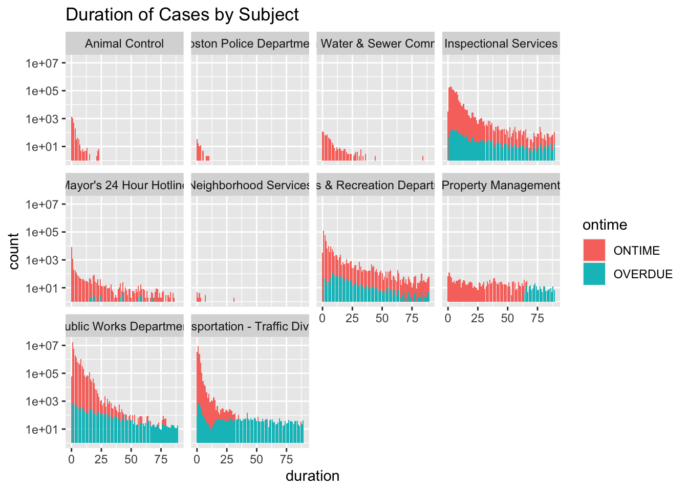
The graph above shows the distribution of duration for each subject. On the y-axis, we are counting the number of cases of a given duration, and showing this on a log scale. By using a log scale, we are able to see in more detail which types of cases have above average durations. Because we are using a log scale, it may appear as though some subjects have a larger proportion of overdue cases than they actually do. Above, we explore in more detail the ontime and case fulfillment rates of each department. From this figure, we can see clearly that most cases have a duration of less than 25 days. Cases under the subjects Animal Control and the Boston Water and Sewer Commission all seem to be fulfilled quickly: nearly all Animal Control cases and most Water and Sewer Commission cases were fulfilled within 25 days. We have very limited data on Neighborhood Services, and most Boston Police Department cases were never closed (the closed rate is roughly 20%, shown above) meaning they do not have a duration. Therefore, we cannot make any claims about the duration of cases of these subjects. It does appear that cases in Property Management have a relatively uniform duration distribution. In other words, it would appear that Property Management cases are just as likely to have shorter durations as they are to have longer durations, whereas cases in most other subjects are more likely to have shorter than longer durations. These results may be exaggerated because we are using a log scale for the y-axis. However, the relative proportion of cases with short durations in Property Management (e.g. duration < 50) is clearly smaller than the same proportion under subjects such as Transportation, Public Works, Inspectional Services, and Parks and Recreation.

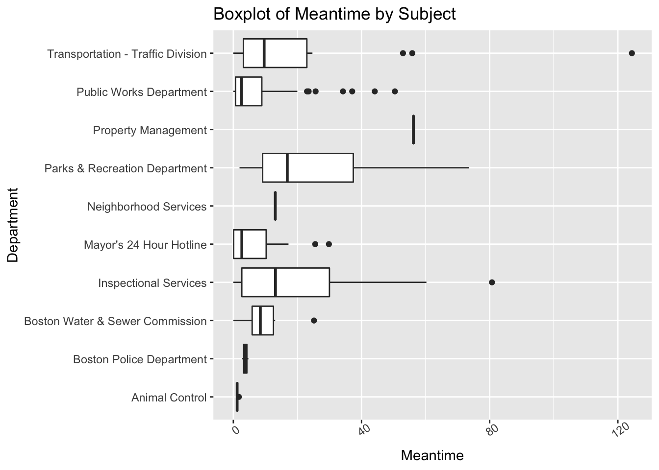
Above we have created a boxplot of meantime by subject. This shows us the overall spread of the duration variable for each subject. This figure shows us similar information as the previous figure, however the boxplot allows us to more easily compare the mean and variance of duration by subject. We see that Inspectional Services and Parks and Recreation have the widest 75% confidence intervals, whereas cases in Public Works and Boston’s Water and Sewer Commission have much narrower confidence intervals, suggesting a smaller variance in the duration of the latter cases. Overall, it is apparent that the spread of duration varies quite a lot depending on case subject.

Modeling

After comparing the AIC values of several models, we find that the best model given our data regresses duration on income, day, and subject (including an interaction term between subject and day). It should be noted that we removed all Boston Police Department cases from our dataset before modeling, because of the extremely limited number of closed cases for this subject. We find no significant relationship between duration and income. There are only 5 terms in our model that are not insignificant: three subject terms for Inspectional Services, Parks and Recreation Department, and Property Management, as well as two interaction terms between subject and day for Inspectional services and Parks and Recreation Department. In other words, we find that the duration of cases is related to the subject of the case for cases in inspectional services, parks and recreation, and property management. Furthermore, we find that case duration varies significantly with time for cases in inspectional services and parks and recreation. The R^2 for this model is 0.1407, meaning roughly 14% of the variation in duration can be explained by the variables included in our model (i.e. day, subject, and income). This means that most of the variation in duration that we see is due to factors not included in our model.

Residual Plot

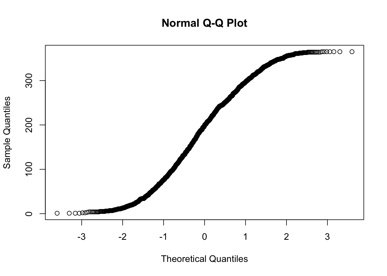
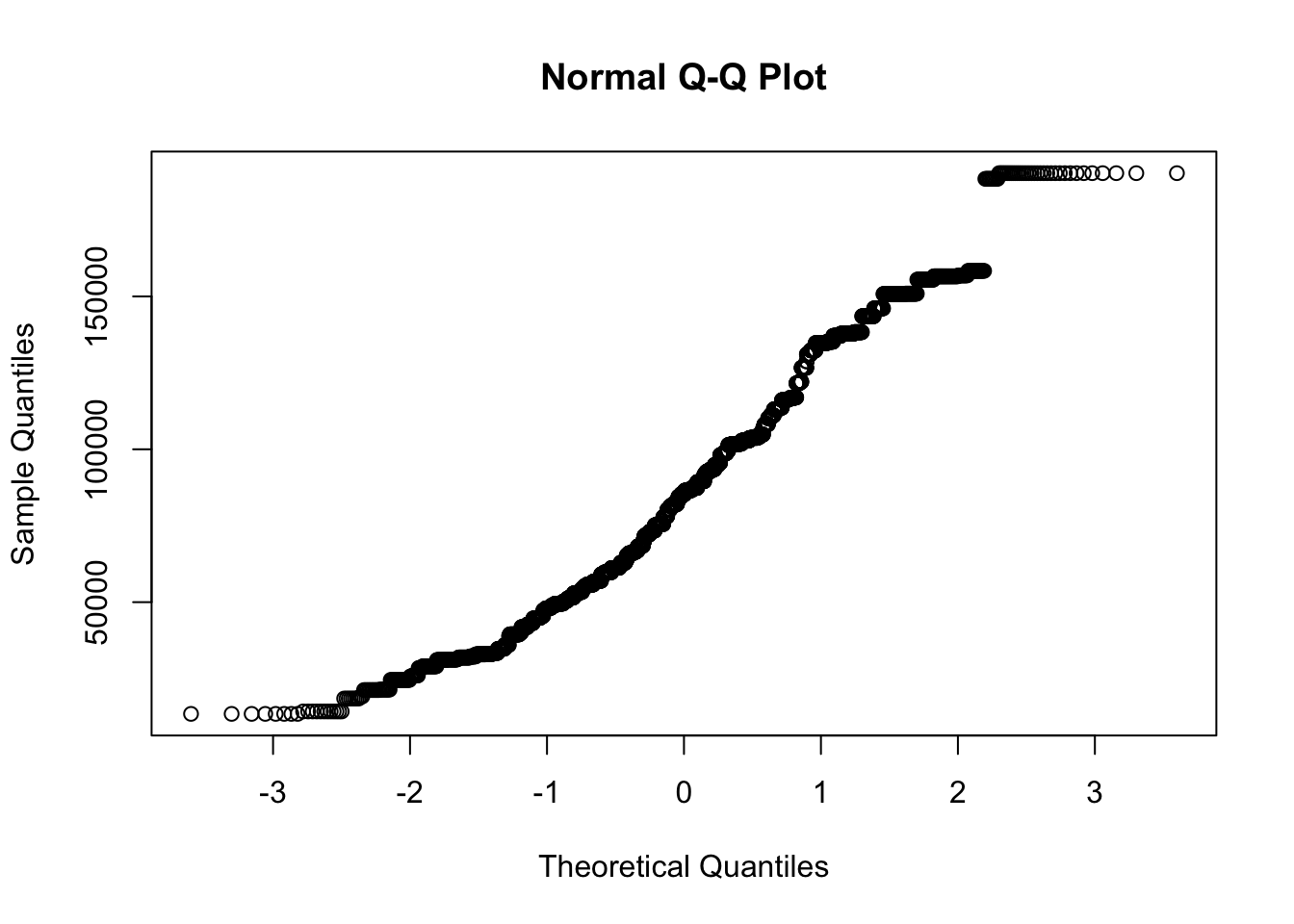
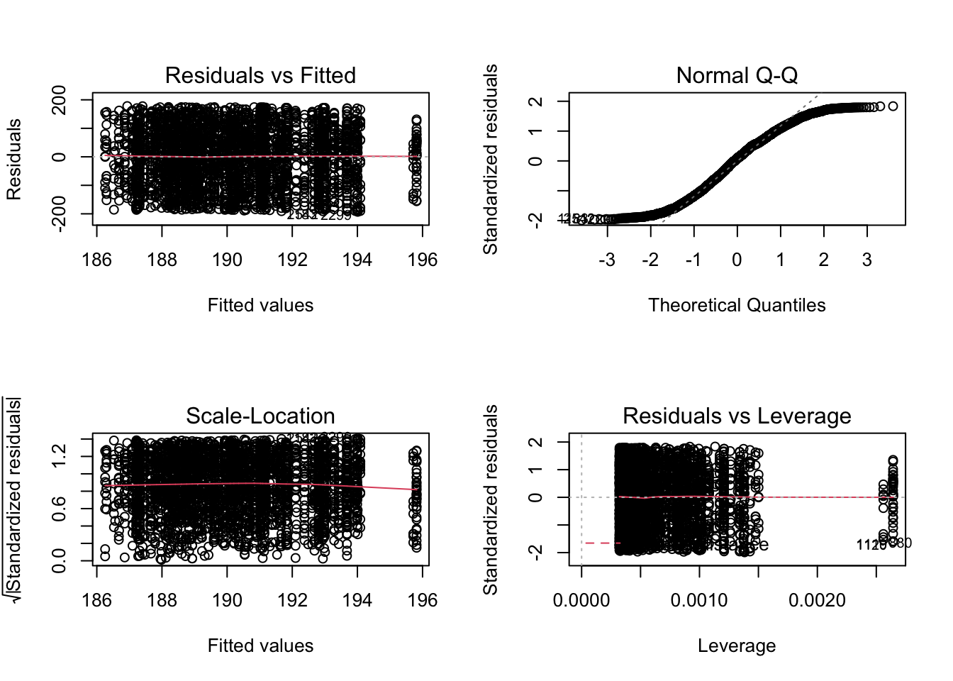For the residual plot, it is showing a similar amount of points on top and below the line, which is indicating that the data is normally distributed. On the other hand, when we look at the normal Q-Q plot, most of the data points are following the 45 degree line except some of the points near the head and tail, but we can still conclude that this is pretty normal. And on the residual vs leverage plot, we can see there are some obvious leverage points/outliers near the end of the line, especially for point 1120, maybe we can consider removing that point and other points around that location.

Multiple Linear Regression

Since we want to know the linear relationship between some of our explanatory variables and response variables, we choose to perform a multiple linear regression. In this case, days, income and Asian race, and the response variable will be duration. And in order to make a better interpretation for these variables, we made an ANOVA table, variance inflation factors, and the correlation matrix between the response variable to other explanatory variables. For the tests that presented in this part, we set the alpha/significant level to 0.05, because top 2.5% and bottom 2.5% of the datas are both important in this case, and 0.05 is a good balance to avoid Type I and Type II errors.

##               [,1]
## [1,]  1.488766e+01
## [2,] -3.644895e-02
## [3,]  2.078334e-06
## [4,]  9.389821e-04

## [1] 2.759316e-08

##    metric        value
## 1     SST 1.920886e+06
## 2     SSE 1.890478e+06
## 3     SSM 3.040823e+04
## 4     MSM 1.013608e+04
## 5     MSE 7.929858e+02
## 6     MST 8.047283e+02
## 7   Fstat 1.278217e+01
## 8   Fcrit 2.608631e+00
## 9 p-value 2.759316e-08

As we can see from the summary statistics, the p-value is less than the alpha level. We have enough evidence to conclude that this model is statistically significant and we can use days, income and asian race as our predictor variables. And we also know that the F-statistic value is larger than the F-critical value, which is indicating we should reject the null hypothesis.(beta1=beta2=beta3=0).

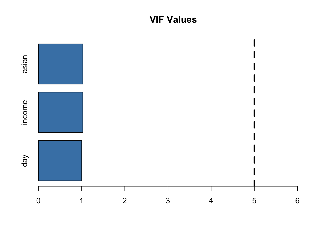
Since we are using more than two predictor variables, we want to avoid multicollinearity in the regression model. So we used the variance inflation factor(VIF) to measure the correlation and strength of correlation between the predictor variable in a regression model. If the VIF value is 1 that means there is no correlation, if the VIF value is between 1 and 5 indicates moderate correlation, and if the VIF value is greater than 5 that indicates potentially severe correlation between these predictor variables. According to our barplot above, it is clear to see that all of the VIF values are near 1, which means we can conclude that they are moderately correlated.

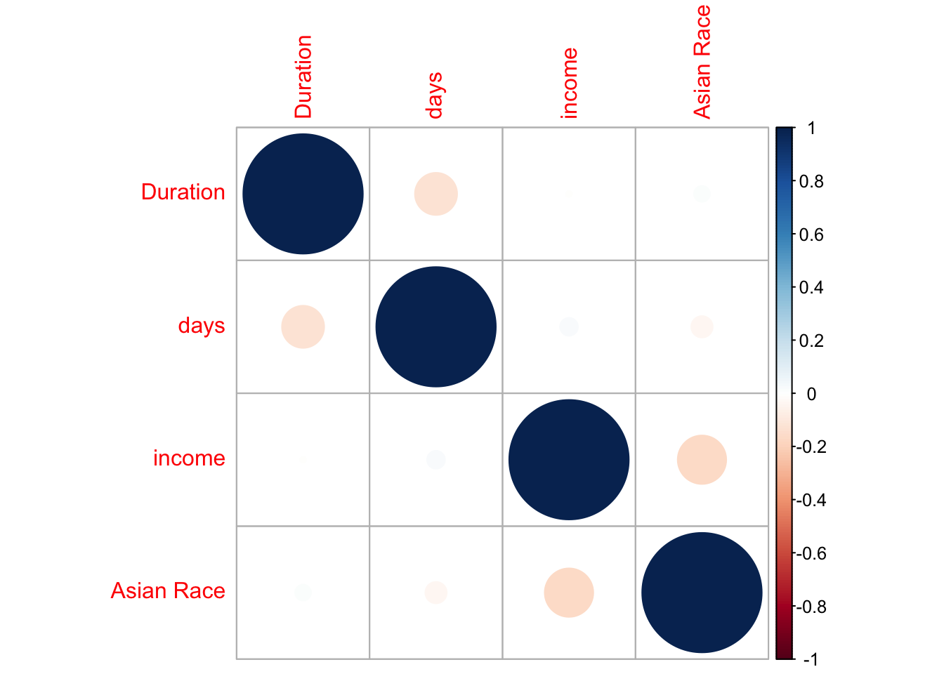
Another way to figure out the correlation between these variables is to make a corrplot, the larger the circle is means the larger correlation. We can see that only duration and days have little correlation with each other.