Combining Datasets

##Loading Data and Packages

First, we load in our data and required packages.

## Warning: package 'sf' was built under R version 4.1.2

## Linking to GEOS 3.9.1, GDAL 3.4.0, PROJ 8.1.1; sf_use_s2() is TRUE

## Warning: package 'tidycensus' was built under R version 4.1.2

## Rows: 273951 Columns: 29

## ── Column specification ────────────────────────────────────────────────────────
## Delimiter: ","
## chr  (20): ontime, case_status, closure_reason, case_title, subject, reason,...
## dbl   (6): case_enquiry_id, fire_district, city_council_district, neighborho...
## dttm  (3): open_dt, target_dt, closed_dt

## 
## ℹ Use `spec()` to retrieve the full column specification for this data.
## ℹ Specify the column types or set `show_col_types = FALSE` to quiet this message.

## Rows: 50000 Columns: 18

## ── Column specification ────────────────────────────────────────────────────────
## Delimiter: ","
## chr  (14): ontime, case_status, case_title, subject, reason, type, queue, de...
## dbl   (1): fire_district
## date  (3): open_dt, target_dt, closed_dt

## 
## ℹ Use `spec()` to retrieve the full column specification for this data.
## ℹ Specify the column types or set `show_col_types = FALSE` to quiet this message.

##Linear Modeling

Here, we have modified our model from last week to account for any perodicity in the relationship between duration and open_dt.

## Warning: Removed 6486 rows containing missing values (geom_point).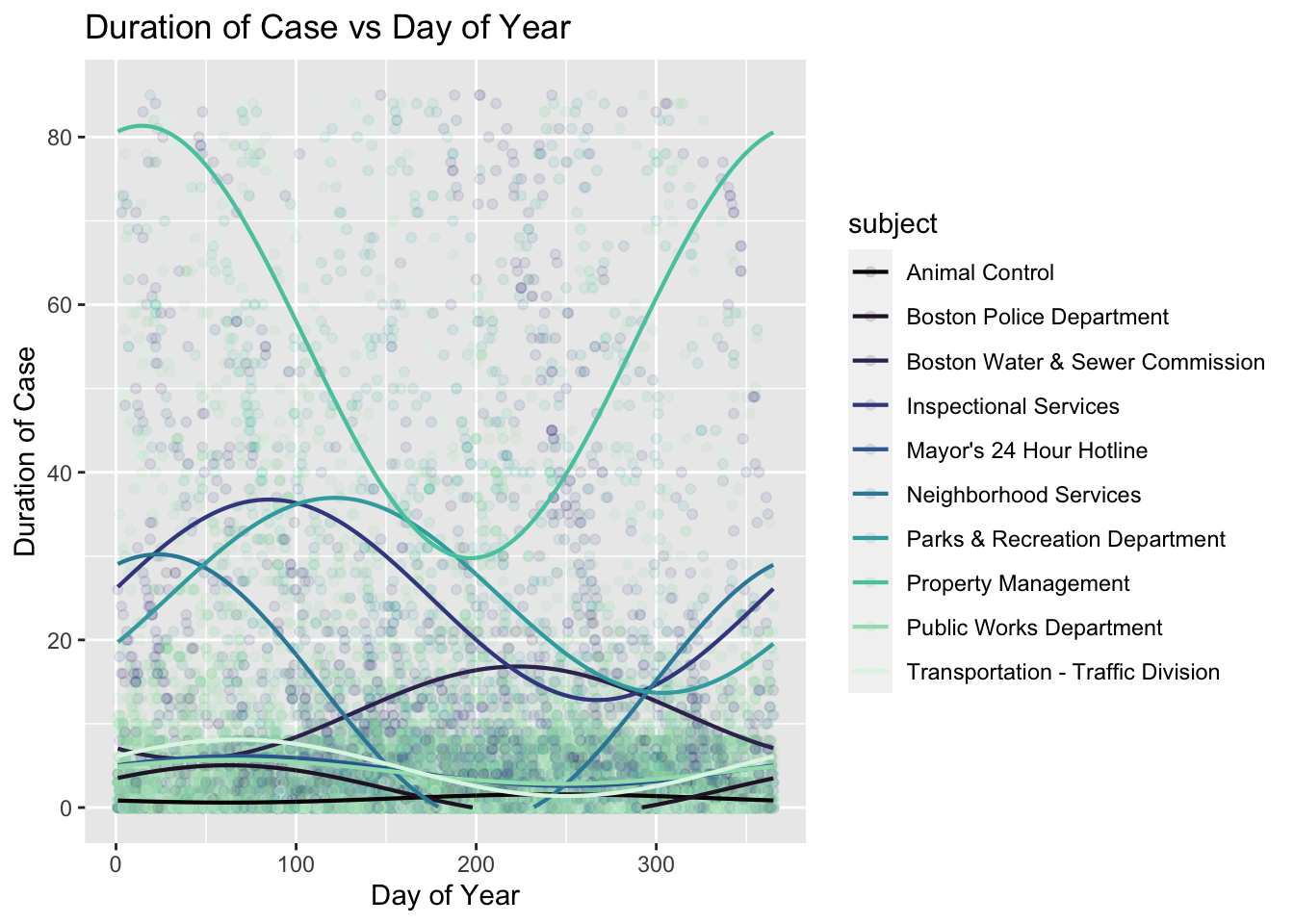

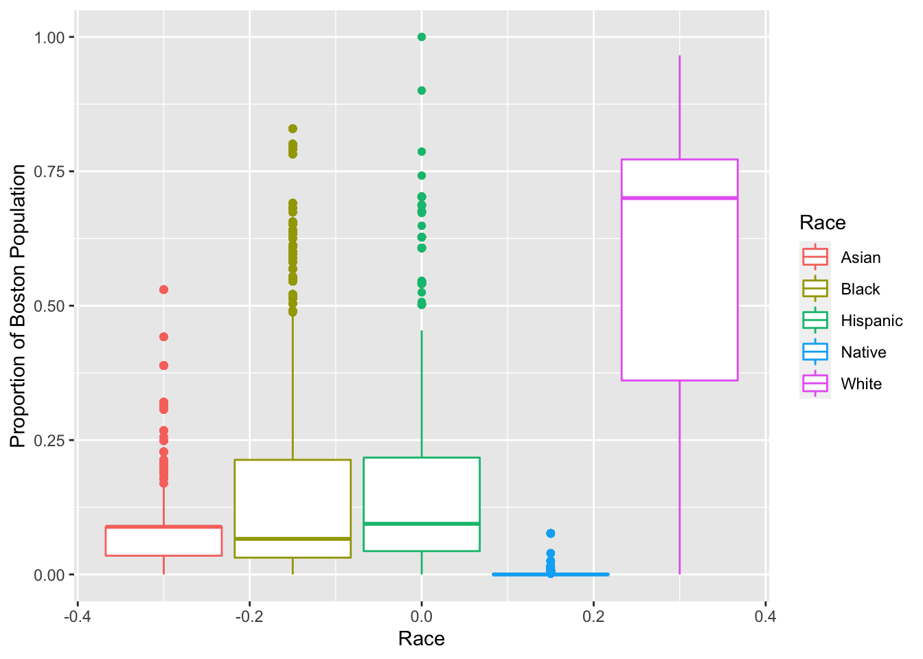
Here, we are combining census information on racial demographics in Boston with our 311 dataset. We are combining the datasets using st_join by matching the coordinates of each 311 case with their corresponding geometry in the census dataset. From the census, we have gathered data on the racial demographics of Boston’s neighborhoods. Eventually, we would like to examine how the duration and type of case does or does not covary spatially with race. For now, we have created a simple boxplot to visualize the distribution (mean and spread/variability) of the data we have on race. We have had some difficulty putting the dataset together. The joint dataset is 140 rows longer than expected (this error margin changes depending on which variables we include). When we include case_enquiry_id in the joint dataset, the columns taken from our 311 dataset are all NAs.

var_tbl <- tidycensus::load_variables(2020, "acs5", cache = TRUE)

options(tigris_use_cache = TRUE)

bos_race <- get_acs(state = "MA", 
                    county = "Suffolk", 
                    geography = "tract", 
                    variables = c(White = "B03002_003",
                                  Black = "B03002_004",
                                  Native = "B03002_005",
                                  Asian = "B03002_006",
                                  Hispanic = "B03002_012"),
                    summary_var = "B03002_001",
                    geometry = TRUE
                    ) %>%
  mutate(proportion = (estimate / summary_est)) %>%
  st_set_crs(4326) %>% 
  st_transform(26986)

## Getting data from the 2015-2019 5-year ACS

## Warning: st_crs<- : replacing crs does not reproject data; use st_transform for
## that

coord_data <- df_311 %>% 
  select(-c(case_enquiry_id, closure_reason, closedphoto, submittedphoto, pwd_district, city_council_district, 
            neighborhood_services_district, ward, precinct)) %>%  
  st_as_sf(coords = c("longitude", "latitude")) %>%
  st_set_crs(4326) %>%
  st_transform(26986) %>% 
  sample_n(5000)

join <- st_join(bos_race, coord_data, join = st_contains)

join %>% 
  group_by(variable) %>% 
  filter(!is.na(proportion)) %>% 
  ggplot() + 
  geom_boxplot(aes(y = proportion, color = variable)) +
  labs(x = "Race", y = "Proportion of Boston Population", color = "Race")