Designing Interactives

##Joint Data EDA

Here, we are using our joint dataset from last week to show the geographic distribution of cases for each of the racial groups in our dataset. We have plotted the log of number of cases per capita, grouped by race. This distribution allows us to look into the correlation between region and race in determining the relative rates of 311 cases in Boston.

suppressPackageStartupMessages(library(tidyverse))
suppressPackageStartupMessages(library(plotly))
library(sf)

## Warning: package 'sf' was built under R version 4.1.2

## Linking to GEOS 3.9.1, GDAL 3.4.0, PROJ 8.1.1; sf_use_s2() is TRUE

library(modelr)
library(tidycensus)

## Warning: package 'tidycensus' was built under R version 4.1.2

df_311 <- read_csv(here::here("dataset-ignore", "311_data.csv"))

## Rows: 273951 Columns: 29

## ── Column specification ────────────────────────────────────────────────────────
## Delimiter: ","
## chr  (20): ontime, case_status, closure_reason, case_title, subject, reason,...
## dbl   (6): case_enquiry_id, fire_district, city_council_district, neighborho...
## dttm  (3): open_dt, target_dt, closed_dt

## 
## ℹ Use `spec()` to retrieve the full column specification for this data.
## ℹ Specify the column types or set `show_col_types = FALSE` to quiet this message.

options(tigris_use_cache = TRUE)

bos_race <- get_acs(state = "MA", 
                    county = "Suffolk", 
                    geography = "tract", 
                    variables = c(White = "B03002_003",
                                  Black = "B03002_004",
                                  Native = "B03002_005",
                                  Asian = "B03002_006",
                                  Hispanic = "B03002_012"),
                    summary_var = "B03002_001",
                    geometry = TRUE
                    ) %>%
  mutate(proportion = (estimate / summary_est)) %>%
  st_set_crs(4326) %>% 
  st_transform(26986)

## Getting data from the 2015-2019 5-year ACS

## Warning: st_crs<- : replacing crs does not reproject data; use st_transform for
## that

coord_data <- df_311 %>% 
  select(-c(case_enquiry_id, closure_reason, closedphoto, submittedphoto, pwd_district, city_council_district, 
            neighborhood_services_district, ward, precinct)) %>%  
  st_as_sf(coords = c("longitude", "latitude")) %>%
  st_set_crs(4326) %>%
  st_transform(26986) %>% 
  sample_n(5000)

join <- st_join(bos_race, coord_data, join = st_contains)

join %>% st_transform(26986) %>% 
  group_by(variable, GEOID) %>% 
  filter(!is.na(variable), !is.na(GEOID), !is.na(proportion)) %>% 
  summarize(n = n()/mean(estimate)) %>% 
  arrange(-desc(GEOID)) %>% 
  ggplot() + 
  geom_sf(aes(fill = log(n))) +
  facet_wrap(~ variable) +
  scale_fill_viridis_c()

## `summarise()` has grouped output by 'variable'. You can override using the `.groups` argument.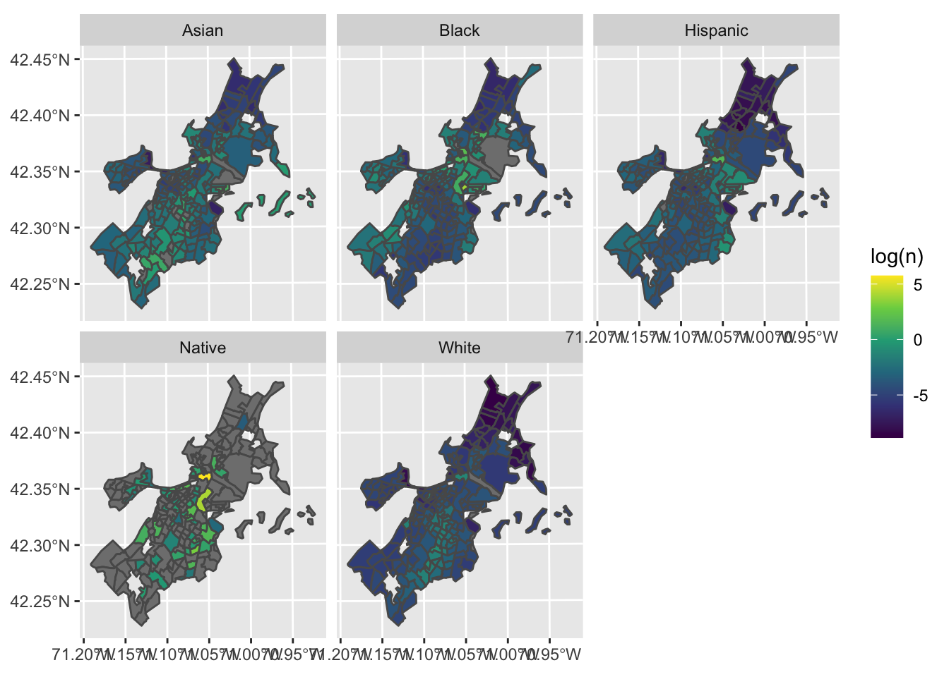

##Shiny App Link https://larcenciel1112.shinyapps.io/interactive_map/