Finalizing Figures and Thesis

##Creating Datasets:

Here, we are finalizing our code for loading and cleaning our datasets.

## ── Attaching packages ─────────────────────────────────────── tidyverse 1.3.1 ──

## ✓ ggplot2 3.3.5     ✓ purrr   0.3.4
## ✓ tibble  3.1.6     ✓ dplyr   1.0.7
## ✓ tidyr   1.1.4     ✓ stringr 1.4.0
## ✓ readr   2.1.1     ✓ forcats 0.5.1

## ── Conflicts ────────────────────────────────────────── tidyverse_conflicts() ──
## x dplyr::filter() masks stats::filter()
## x dplyr::lag()    masks stats::lag()

## Linking to GEOS 3.9.1, GDAL 3.4.0, PROJ 8.1.1; sf_use_s2() is TRUE

## 
## Attaching package: 'plotly'

## The following object is masked from 'package:ggplot2':
## 
##     last_plot

## The following object is masked from 'package:stats':
## 
##     filter

## The following object is masked from 'package:graphics':
## 
##     layout

## Loading required package: viridisLite

## Rows: 273951 Columns: 29

## ── Column specification ────────────────────────────────────────────────────────
## Delimiter: ","
## chr  (20): ontime, case_status, closure_reason, case_title, subject, reason,...
## dbl   (6): case_enquiry_id, fire_district, city_council_district, neighborho...
## dttm  (3): open_dt, target_dt, closed_dt

## 
## ℹ Use `spec()` to retrieve the full column specification for this data.
## ℹ Specify the column types or set `show_col_types = FALSE` to quiet this message.

## Getting data from the 2015-2019 5-year ACS

## Warning: st_crs<- : replacing crs does not reproject data; use st_transform for
## that

## Getting data from the 2016-2020 5-year ACS

## Warning: st_crs<- : replacing crs does not reproject data; use st_transform for
## that

##Data Exploration and Figures:

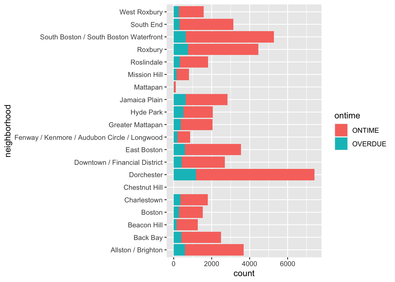
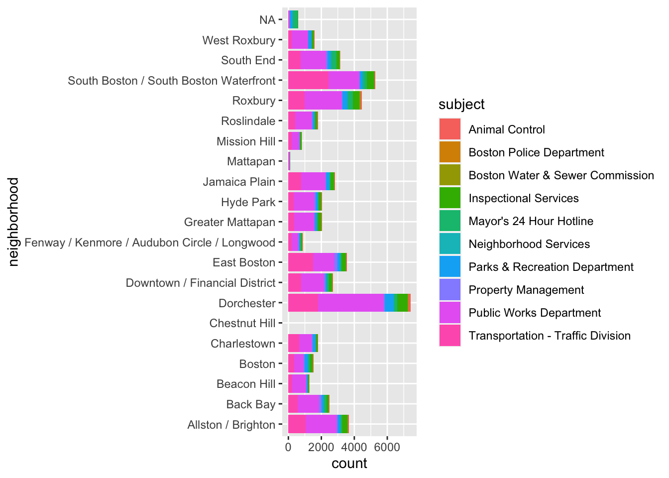
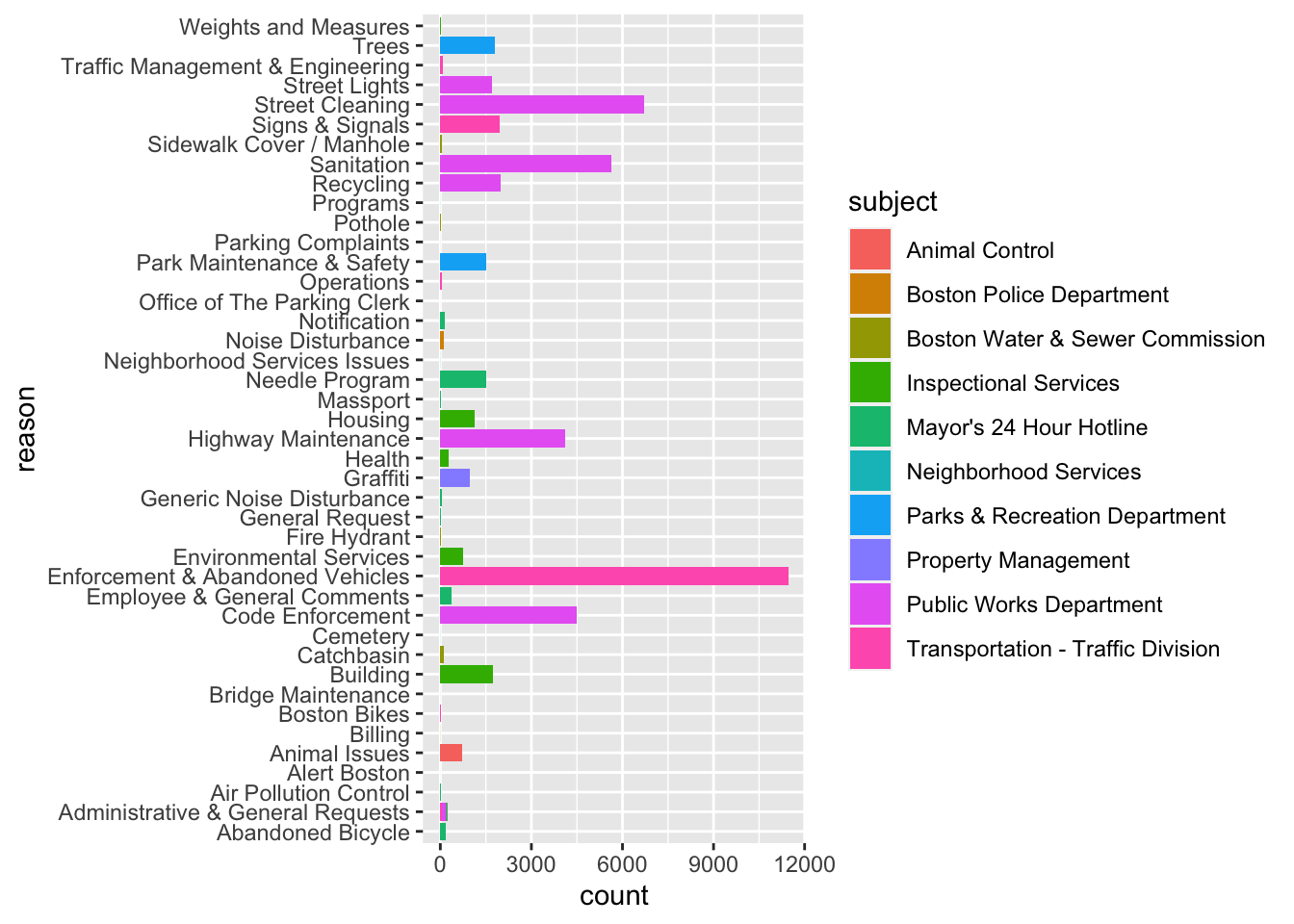
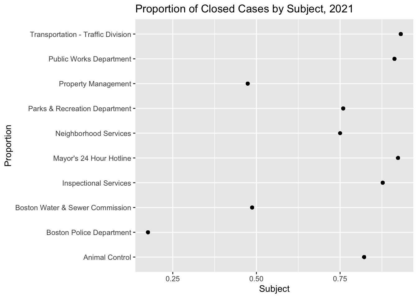
Here, we have compiled and begun cleaning the figures from our EDA that we would like to use on our website.

#BASIC EDA

## Don't know how to automatically pick scale for object of type difftime. Defaulting to continuous.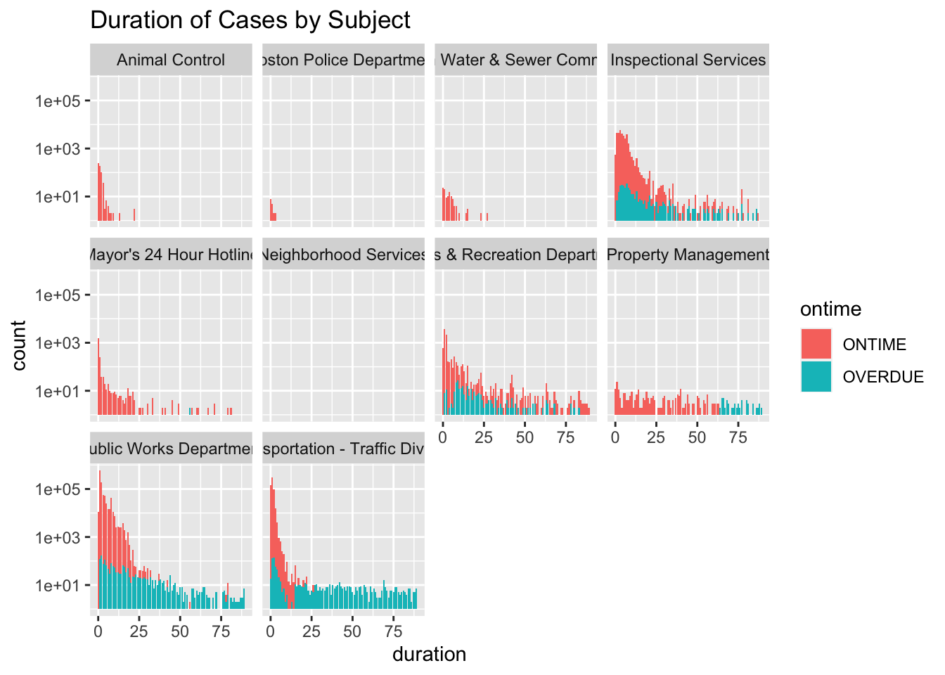

#MAPS

#map of racial demographics
join %>% group_by(variable.x, GEOID.x) %>% 
  ggplot(aes(fill = estimate.x/summary_est)) +
  geom_sf() +
  labs(title = "Map of Boston Sub-Districts Colored by Population, Grouped by Race") +
  facet_wrap(~ variable.x) +
  scale_fill_viridis_c()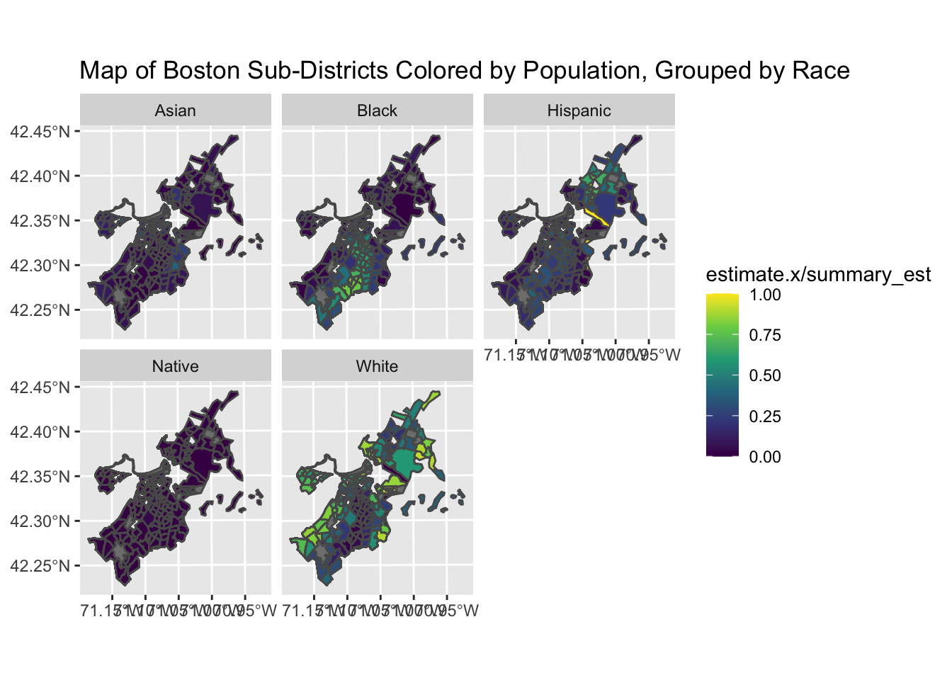

#map of log number of cases
join %>% group_by(GEOID.x) %>% 
  summarize(n = n()) %>% 
  ggplot(aes(fill = log(n))) +
  geom_sf() +
  labs(title = "Map of Boston Sub-Districts Colored by the log of Number of Cases") +
  scale_fill_viridis_c()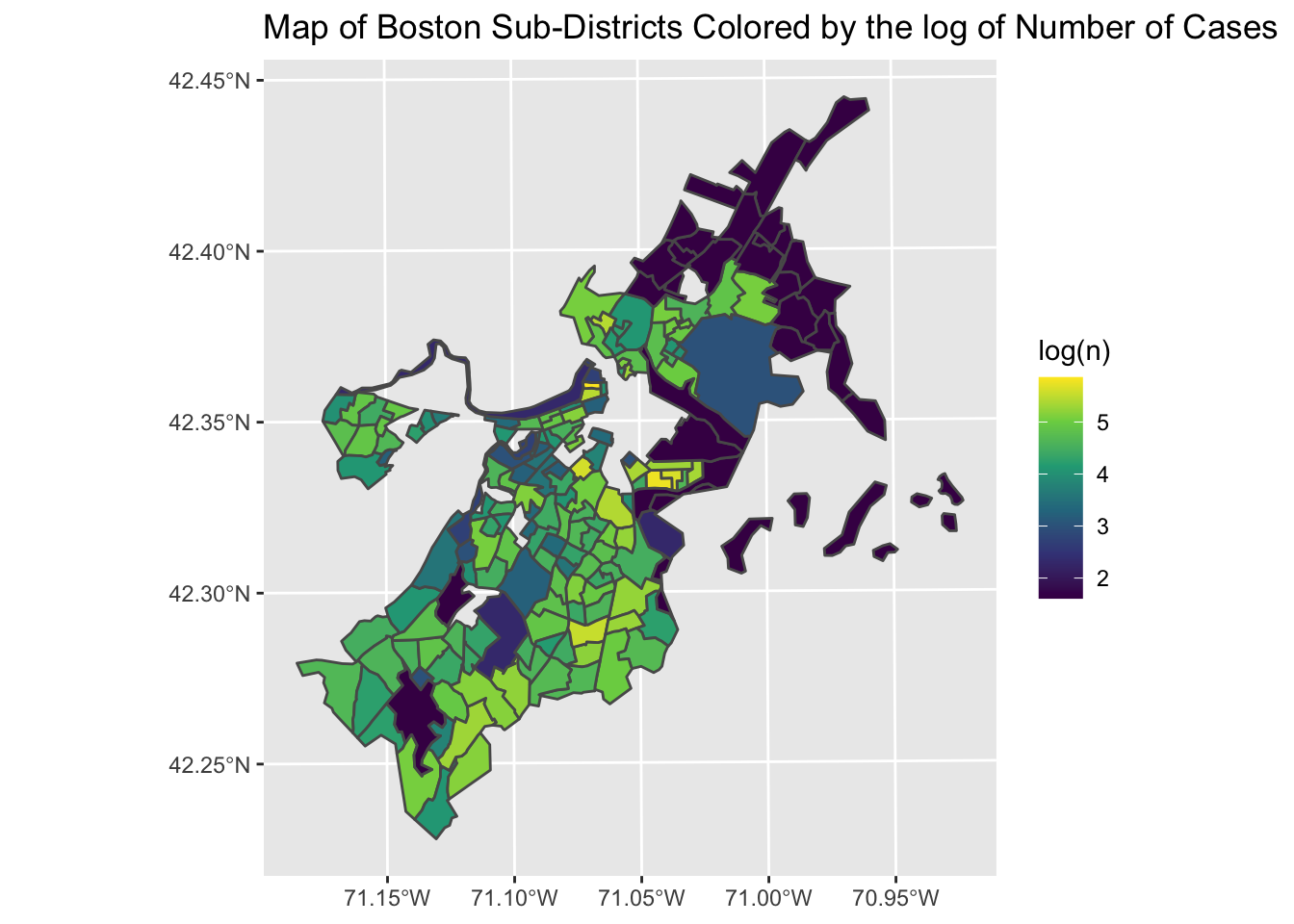

#map of income distribution
bos_income %>% group_by(GEOID) %>% 
  ggplot(aes(fill = (estimate))) +
  geom_sf() +
  labs(title = "Map of Boston Sub-Districts Colored by Income") +
  scale_fill_viridis_c()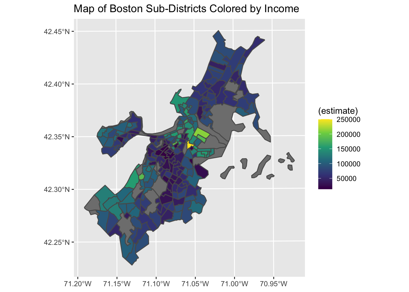

##Thesis

For the topic of our thesis, we are interested in examining the effects of location, racial demographics, income, day of year, and case subject on the duration of 311 cases in Boston. We plan to finalize our thesis statement as soon as we have a finalized model incorporating data from both datasets.